Multi-GPU Physics Based Hamiltonian Monte Carlo
HMC is widely used in probabilistic programming, as part of fitting many-parameter models. Our implementation — created from scratch — is scalable, portable and based on Physics.
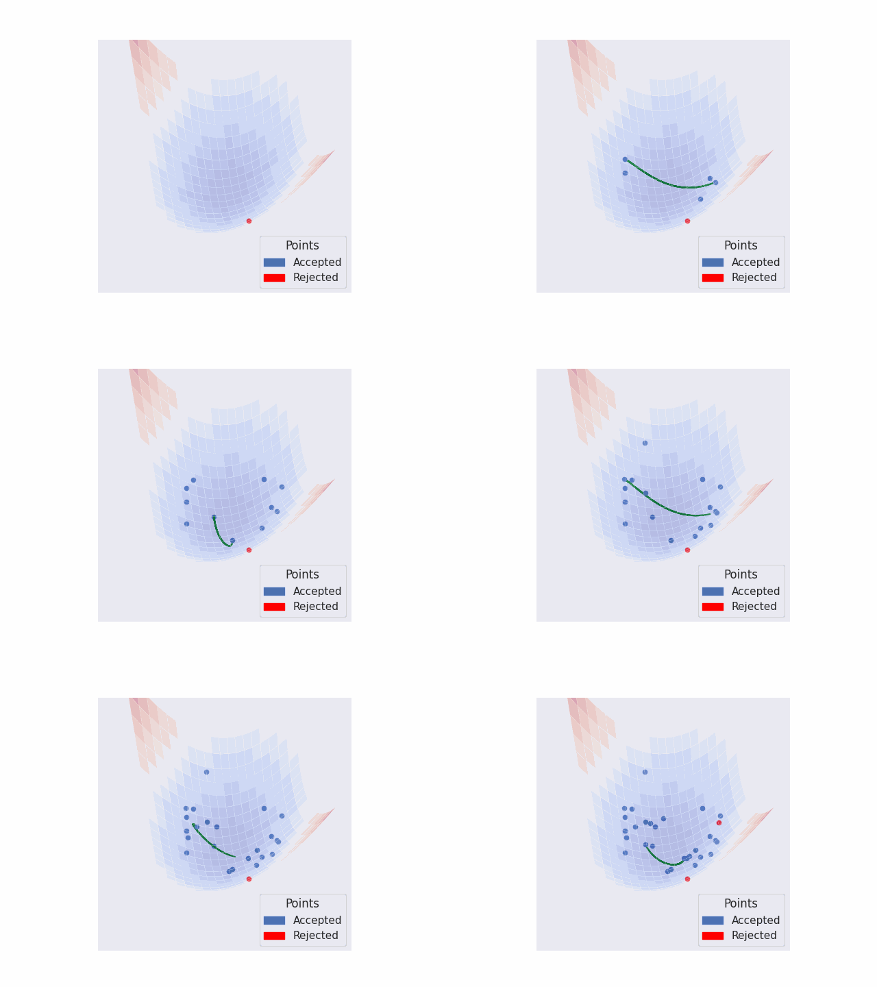 |
|---|
| HMC exploring a bowl-shaped potential. Accepted proposals are shown in blue, rejected ones in red. |
Generating samples from a given probability distribution function is a surprisingly difficult task, and Hamiltonian Monte Carlo (HMC) solves this challenge in an elegant way. HMC is widely used in probabilistic programming packages, such as Stan and Numpyro, which use the algorithm to sample parameters from posterior probability distributions, which govern the distribution of model parameters given some data. The size and number of parameters of some statistical models, such as those in epidemiology, justifies parallelized HMC schemes.
There were two principal goals for this project. First, we had to implement from scratch in Python the HMC algorithm as presented and discussed in previous works. For such a purpose, we opted for a physics based approach, as this allowed for a more intuitive interpretation and future extension of the method. We assumed we were given a system with particles moving in a multidimensional space and these do not interact with each other. In addition, each particle had its own mass and the system could be heated up and cooled down by considering the temperature as a parameter.
Secondly, we adapted our implementation with the goal of it being able to run on multi-CPU or GPU clusters by simply changing one line of code.
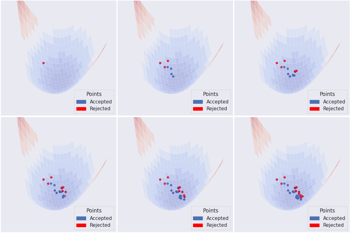 |
|---|
| Proposals generated by the Metropolis-Hastings algorithm. Note the high rejection rate and high correlation, even with 2 dimensions. |
Theory
To begin with, let us assume that we have a model, and some data which is supposed to be explained by the model. Through Bayesian inference the probability distribution of the model parameters can be deduced. Generating parameter samples from this distribution is difficult or impossible via inverse transform sampling, but can be done via HMC.
Bayes Rule
We recall that Bayes theorem states that given the prior probability \(p(\mathbf{q})\) and a set of observed data \(y\) whose likelihood is \(p(y \mid \mathbf{q})\), then the posterior probability \(p(\mathbf{q} \mid y)\) is
\[p(\mathbf{q} \mid y) = \frac{p(\mathbf{q}) \, p(y \mid \mathbf{q})}{p(y)},\]where \(p(y)\) is a normalizing constant, which may be ignored. Typically, \(p(\mathbf{q} \mid y)\) corresponds to the distribution we want to sample from, which we will call \(\pi(q)\) from now on. HMC samples from this distribution for the parameters, as outlined below. This is done to calculate expectation values for the parameters of the distribution, along with standard deviations.
Markov Chain Sampling Methods
Let us assume we are interested in generating samples from a probability distribution function or density function \(\pi(\mathbf{q})\) with parameter \(\mathbf{q}\) on a \(D\)-dimensional space, \(Q\). Furthermore, \(\pi(\mathbf{q})\) is not easily invertible or is not available in closed form.
The subset \(T \subset Q\) where the product \(\pi(\mathbf{q}) \, d\mathbf{q}\) such that \(\mathbf{q} \in T\) is non-negligible is called the typical set. This region is where we want to sample from. Notably the volume of \(T\) relative to the region surrounding \(T\) decreases as \(D\) increases.
There exist many sampling techniques to generate points from \(\pi(\mathbf{q})\) and one of the most widely used techniques is a class of statistical methods called Markov Chain Monte Carlo (MCMC). These methods, intuitively, consist of randomly navigating through the space spanned by parameter \(\mathbf{q}\), commonly called parameter space.
Most MCMC methods work by generating the proposals for the next sample (\(\mathbf{q}_{n+1}\)) in proximity to the current sample (\(\mathbf{q}_n\)). For instance, the Gaussian Metropolis-Hastings method involves taking a random Gaussian step in parameter space to get the next proposal, which we denote by \(\mathbf{q}^\prime\). The proposal is then accepted or rejected with probability \(\pi(\mathbf{q}^\prime)/\pi(\mathbf{q}_n)\). The rejection of samples at a lower probability density causes the walk to “stay on track”, and for computational resources to be focused on the typical set, where the density of the target distribution is significant.
This simple Metropolis-Hastings method, shown above, struggles with high-dimensional distributions, when \(D\) is large, as the volume surrounding \(T\) is much larger than the volume of \(T\) itself, meaning most proposals are in regions of \(Q\) where \(\pi(\mathbf{q}) \, d\mathbf{q}\) is negligible and are, therefore, rejected. This is not efficient at best and totally infeasible if \(D\) is sufficiently high.
From Markov Chains to Particles
This is where HMC steps in. Work on the random motion of smoke particles in air (Brownian motion) by Einstein and others established that the motion of particles in a gas can be modeled using Markov chains. Inverting this, some Markov chains can be considered as particles. Suppose that we are given a particle whose position vector \(\mathbf{q}\) is on a \(D\)-dimensional space; keep in mind that \(\mathbf{q}\) is the parameter we are interested in. HMC doubles the parameter space \(Q\) by adding an extra parameter, which we refer to as momentum, \(\mathbf{p}\). Then, we have a joint probability distribution function depending on \(\mathbf{q}\) and \(\mathbf{p}\), that is, \(\pi(\mathbf{q}, \mathbf{p}) = \pi(\mathbf{p} \mid \mathbf{q}) \, \pi(\mathbf{q})\).
Notably, in physics we often sample from the canonical distribution, which is given by
\[\pi(\mathbf{q}, \mathbf{p}) = \exp\bigl(-H(\mathbf{q}, \mathbf{p})\bigr),\]where \(H(\mathbf{q}, \mathbf{p})\) is the Hamiltonian or energy value at \((\mathbf{q}, \mathbf{p})\).
We notice that \(H(\mathbf{q}, \mathbf{p})\) can be written as the sum of kinetic \(K(\mathbf{p}, \mathbf{q})\) and potential energy \(V(\mathbf{q})\) as follows:
\[H(\mathbf{q}, \mathbf{p}) = -\log \pi(\mathbf{q}, \mathbf{p}) = -\log \pi(\mathbf{p} \mid \mathbf{q}) - \log \pi(\mathbf{q}) = K(\mathbf{p}, \mathbf{q}) + V(\mathbf{q}).\]This means that each point in the parameter space is assigned a potential energy \(V(\mathbf{q}) = -\ln{\pi(\mathbf{q})}\). To illustrate this, imagine a 2D Gaussian distribution \(\pi(\mathbf{q}) = \exp(-q_1^2 - q_2^2)\) (lacking normalization). This has a bowl shaped parabolic potential energy function \(V(\mathbf{q}) = q_1^2 + q_2^2\). We set \(K(\mathbf{p}, \mathbf{q}) = (\mathbf{p}^{T} \cdot \mathbf{p}) / 2m\). Such a choice of \(K(\mathbf{p}, \mathbf{q})\) is usually implemented as discussed in the references. Besides, we state that the Hamiltonian captures the “geometrical information” of \(T\) and that \(K(\mathbf{p}, \mathbf{q})\) is non-unique.
To go from one sample to the next, we give the “particle”, whose mass is \(m\), a random momentum \(\mathbf{p}\) from a Maxwell-Boltzmann distribution, which approximates the motion of particles in an ideal gas. In practice this means momentum is drawn from a multivariate normal distribution with a mean of zero and the standard deviation for each coordinate as given below:
\[\sigma_{p_i}^2 = \sigma_{p_{i+1}}^2 = \dots = m k_b T,\]for \(i = 1, \dots, D-1\).
We then simulate the evolution of the system for a certain number of time-steps, which requires solving Hamilton’s equations for \(\mathbf{p}, \mathbf{q}\). This is done using a symplectic integrator — which conserves the Hamiltonian, i.e. energy — such as the leapfrog method. We recall that the force \(F\) acting upon the particle is the negative of the gradient of the potential with respect to position; that is
\[F = -\nabla V(\mathbf{q}).\]To concretize the evolution, imagine a hockey puck being given a random momentum in a large, parabolic bowl. In an ideal world, this method of generating proposals negates the need for an acceptance/rejection step, for reasons outlined in the references. However, in reality, a small number of proposals are rejected due to numerical integration errors. Nonetheless, with a suitable time-step most proposals are accepted and samples have a lower correlation than those produced by Metropolis-Hastings.
Methods
The implementation was made using Google’s jax, which is NumPy accelerated on GPU. Jax features just-in-time compilation, automatic differentiation and parallelization of evaluation by means of vectorization via vmap. MPI was used to run the program on multiple GPUs, where vmap was used to run multiple particles in parallel as illustrated below.
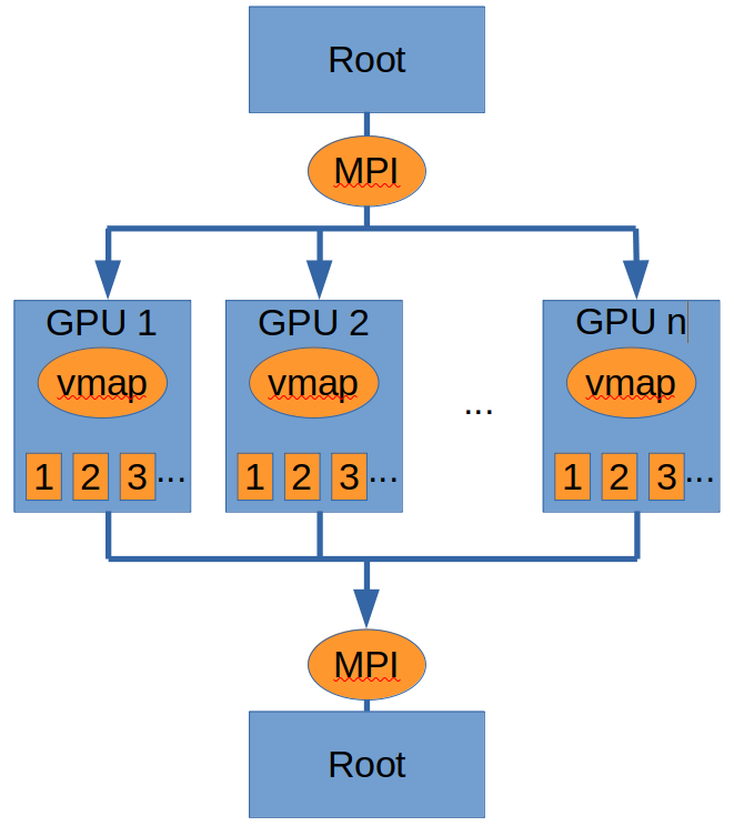 |
|---|
| Parallel architecture. |
Numpyro played an important role in the project, as it was used to set up the probabilistic models and calculate the log posterior distribution from observations. The posteriors were then sampled from using our HMC kernel.
Results
We achieved the initial goal of fitting probabilistic models on multiple GPUs. The implementation is also extremely portable, as it can be run on CPUs or GPUs easily, with no requirement for all GPUs to be of the same architecture. The figure below shows the scaling of the implementation with the number of particles on a single CPU, a single GPU and two GPUs of different architectures.
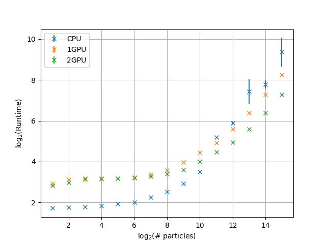 |
|---|
| A GTX 1080Ti and RTX 3050 were used, inferring the bias of two coins. |
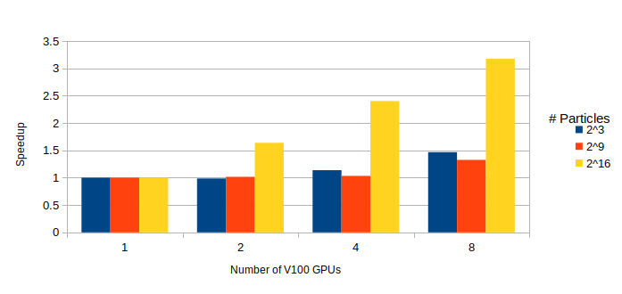
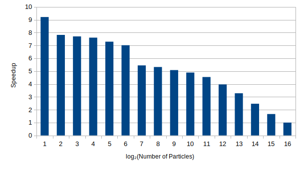
The speedup of the algorithm with the number of V100 GPUs used is plotted below, whilst the change in run time on one GPU as the number of particles increases is shown after it. The weak scaling in both plots is a consequence of the model being far too small to fully utilize the GPUs, meaning much of the run time is overhead. We limited ourselves to small models which can be solved analytically because this allowed us to verify the correctness of the results obtained with our implementation.
 |
|---|
| Speedup vs number of V100 GPUs for various numbers of particles. |
 |
|---|
| Speedup vs Number of Particles on one V100 GPU. |
Discussion/Conclusions
Overall we are pleased with our progress and the results so far have been promising. In the future, we plan to fit some larger models and explore how tuning physical parameters can affect our performance.
One promising avenue is simulated annealing. Let us say we have a bimodal distribution function (i.e. a pdf with two local maxima). To start we set momentum’s with a high temperature, meaning the entire potential landscape (and hopefully each mode) is more readily explored. We gradually lower the temperature before generating samples from the chains, so the tails of the distribution are not over represented.
Also, it is worth noting that current results have been obtained with code that has not yet been optimized. Profiling reveals significant host-device communication which, in combination with the small models used, explains the limited scalability observed so far. Eliminating these transfers and increasing the model size in the coming weeks should lead to major improvements in scalability.
Project details
- Project title: Multi-GPU Physics Based Hamiltonian Monte Carlo (PRACE SoHPC Project ID 2216)
- Site: Hartree Centre — STFC, United Kingdom
- Authors: Bruno Rodriguez Carrillo (Mexico), Thomas Warford (UK)
- Mentor: Anton Lebedev, Hartree Centre — STFC, UK
- Software applied: jax, mpi4jax, numpyro
Acknowledgements
Thanks to Anton Lebedev for mentorship and contribution to code. Thanks to Hartree Centre and PRACE.
References
- Stan Reference Manual, Version 2.30, Chapter 15.
- Numpyro Documentation.
- Betancourt, M. (2017). A conceptual introduction to Hamiltonian Monte Carlo. arXiv preprint arXiv:1701.02434.
- Hoffman, M. D., & Gelman, A. (2014). The No-U-Turn sampler: adaptively setting path lengths in Hamiltonian Monte Carlo. J. Mach. Learn. Res., 15(1), 1593-1623.