Discovering Digits with Convolutional Autoencoders

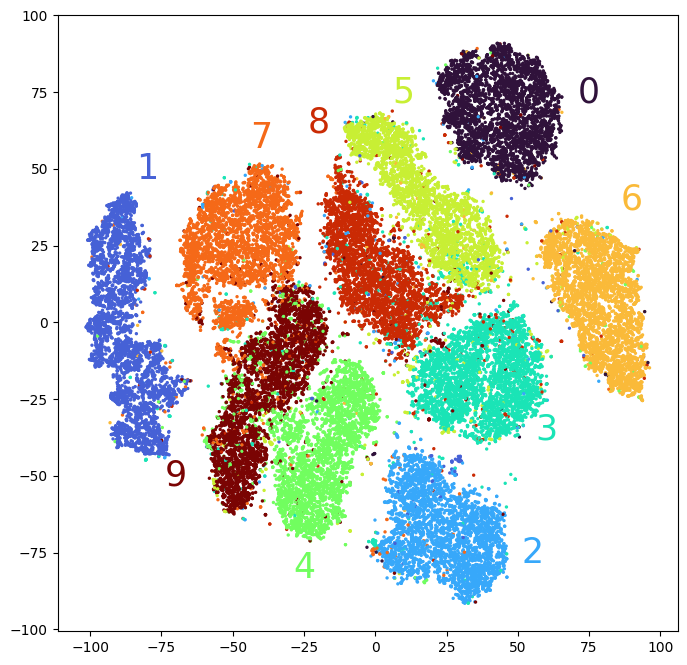
Each colour corresponds with a different digit — the seperation between digits has been learned!

Autoencoders are neural networks which take an image as input, and are trained to reproduce that image. Their usefulness comes from from their middle layer activations having fewer dimensions than the original data, effectively compressing the input data. These activations can be thought of as vectors in a latent space, and the positions of the vectors in this space can be really interesting.

Although not created with an autoenoder, the learned vectors of words created by word2vec illustrate how interesting this can be, for instance “king=queen-woman+man”.

The Architecture

Convolutional layers are great at extracting features from images, and by making stride-2 convolutions the width and height of images is halved.

Here’s the pytorch code for a simple convolutional layer, simply a convolution followed by an optional activation layer.

def conv(
    ni, # input channels (3 for rgb image)
    nf, # output channels
    ks=3, # kernal size (ks * ks)
    act=True): #whether we add an activation layer

    layers = [nn.Conv2d(ni, nf, ks, stride=2, padding=ks//2)]
    if act:
        layers.append(nn.ReLU())
    
    return nn.Sequential(*layers)

Many of these convolutional layers put together forms an encoder, which generates the latent representation.

Here’s a “deconvolutional” layer. The upsampling increases the width and height of images by 2 whilst the stride-1 convolution has no effect on image dimensions.

def deconv(
    ni, # input channels (3 for rgb image)
    nf, # output channels
    ks=3, # kernal size (ks * ks)
    act=True): #whether we add an activation layer)
    
    layers = [nn.UpsamplingNearest2d(scale_factor=2), 
                nn.Conv2d(ni, nf, ks, stride=1, padding=ks//2)]
    
    if act: layers.append(nn.ReLU())
    
    return nn.Sequential(*layers)

A series of deconvolutional layers together serves as our encoder, building up the reproduced image from our latent representation.

Here’s the full architecture:

class Autoencoder(nn.Module):
    def __init__(self, n_latent=128):
        super().__init__()
        self.encode = nn.Sequential(
            nn.ZeroPad2d(2), # 32x32
            conv(3, 4), # 16x16
            nn.Conv2d(4, 4, 3, stride=1, padding=1), # 16x16
            nn.ReLU(),
            conv(4, 8), # 8x8
            conv(8, 16), # 4x4
            nn.Flatten(),
            nn.Linear(16*4*4, n_latent),
            nn.Tanh()
        )
        
        self.decode_linear=nn.Sequential(
            nn.Linear(n_latent, 16*4*4),
            nn.ReLU()
        )
        
        self.decode = nn.Sequential(
            nn.ReLU(),
            deconv(16, 8), # 8x8
            deconv(8, 4), #16x16
            nn.Conv2d(4, 4, 3, stride=1, padding=1), # 16x16
            nn.ReLU(),
            deconv(4, 3, act=False), #32x32
            nn.ZeroPad2d(-2), #28x28
            nn.Sigmoid()
        )
        
    
    def forward(self, x):
        output = self.encode(x)
        output = self.decode_linear(output)
        output = output.view(-1, 16, 4, 4)
        return self.decode(output)

Note the addition of a linear layer and Tanh activation to the encoder. I opted to use Tanh to make the latent vectors easier to work with.

You can check out the notebook here: https://www.kaggle.com/code/thomaswarford/mnist-autoencoder-clustering

Results

The autoencoder was trained on the MNIST handwritten digits dataset, with a latent vector of size 128.

Here are the resulting reproductions of letters:

Original and reproduction of the letter 7.

Original and reproduction of letter 9.

Now our autoencoder is trained, we can use the encoder to “vectorize” images. t-SNE let’s us visualize these length-128 vectors in 2 dimensions. Here is the resulting plot, where each colour represents a different digit.

There we go! The separation between different digits is quite impressive, considering we never told the network the labels explicitly.

Improvements

Considering the simplicity of this architecture, it does pretty well. However, applying autoencoders to larger, more complicated images will require some refinements.

Currently my lab partner and I are training an autoencoder to recreate band structure plots similar to the one below and are getting blurry white images as a result.

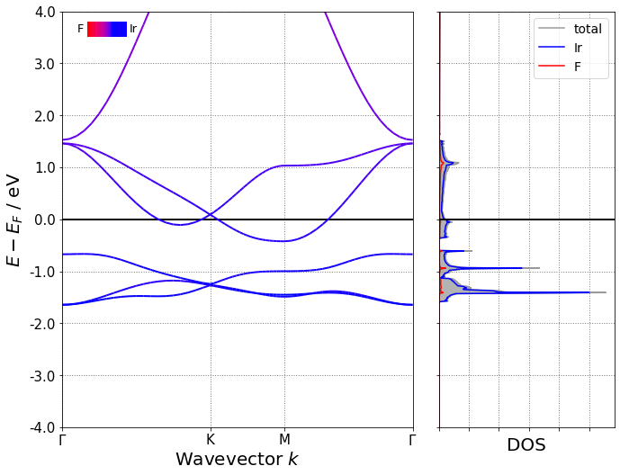
This might suggest that our activations are tending towards zero as you go through the layers — this could be fixed by batch normalisation or LSUV. We’re also going to look at ResNet architectures for inspiration.

Acknowledgements

Thanks for reading. I learnt about autoencoders, including the (de)convolutional layers above, from fast.ai, as well as the tricks I’ll need to make them better. The kaggle notebook linked above uses some of Evan Anders’ code to load in the data.